
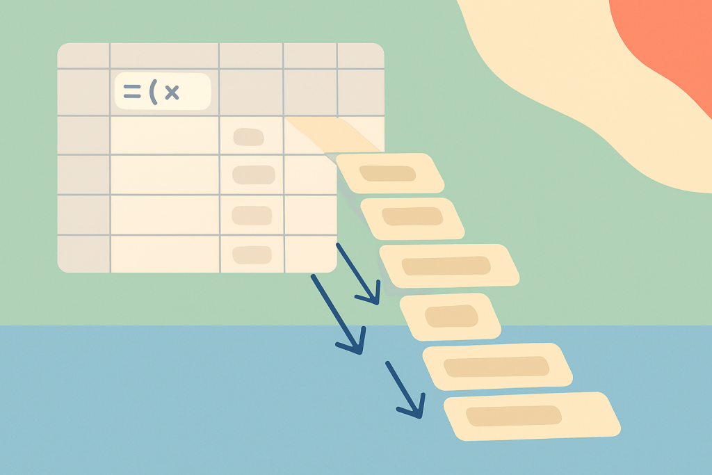
The fill-handle habit is so ingrained it hides its cost. A month-end refresh: filter out old rows, drag the invoice numbers again, then chase the two people who edited a copy before the drag. A quarterly report: extend the date column by hand, remember the working days shift when a holiday lands mid-week. Each pass is cheap on its own. The sheet quietly breaks the moment somebody inserts a row and forgets to re-fill. SEQUENCE replaces that pattern with a single formula that spills across the range you ask for and recalculates when the arguments change. The maintenance step disappears with it.
Why dragging the fill handle keeps costing you time
Fill-handle sequences are static. The instant the underlying count changes — a new customer, a shorter month, an added workday — you either re-drag or accept broken references downstream. Nothing warns you. The formula that consumed the sequence still returns a value, just against the wrong length.
SEQUENCE moves the count into the formula itself. Instead of “start at 1001 and drag to row 47,” you write the intent: give me 47 rows starting at 1001, stepping by 1. If the row count comes from a cell — a COUNTA against the source column, a table row count, an explicit input — the range grows or shrinks automatically the next time the sheet recalculates. Insert a customer, the ID column extends. Delete two, it contracts. Nothing on your end.
#NAME? for the formula.
That one trade — a single formula for a live count — replaces three habits at once: hand-typed invoice numbers, hard-coded month headers, and helper columns whose only purpose is a ROW() arithmetic trick pretending to be a counter. Every workbook has a few of each, and each one is a small liability the next time somebody inserts a row above them.
The four arguments and what happens when you skip them
The signature is =SEQUENCE(rows, [columns], [start], [step]). Only rows is required; the other three default to 1. That gives four common shapes with almost no typing, and the differences show up cleanly in a grid.
| A | B | C | |
|---|---|---|---|
| 1 | Formula | Output shape | Reads as |
| 2 | =SEQUENCE(6) | 6 rows × 1 col | 1..6 down |
| 3 | =SEQUENCE(1, 6) | 1 row × 6 cols | 1..6 across |
| 4 | =SEQUENCE(5, 4) | 5 × 4 grid | 1..20 row-first |
| 5 | =SEQUENCE(5, 1, 1001, 1000) | 5 rows × 1 col | 1001, 2001, … 5001 |
Two shape rules matter for anything more complex. The grid fills by row first — row 1 gets values 1 through cols, row 2 gets cols+1 through 2×cols, and so on. And step accepts negatives: =SEQUENCE(10, 1, 10, -1) counts down 10 to 1 in a single column. See Microsoft’s official SEQUENCE reference for the full argument table.
Number series patterns that ship as one formula
Once the argument shapes click, several familiar workbook habits collapse into a single cell. The examples below are the ones that pay for themselves fastest.
Invoice or ticket IDs that grow with the source table. Replace a helper column that concatenates a prefix with ROW()-1:
="INV-"&TEXT(SEQUENCE(COUNTA(Table1[Customer])), "0000")COUNTA reads how many customers the table has right now; SEQUENCE emits that many integers; TEXT pads to four digits. Add a customer and INV-000N+1 appears without touching the ID column.
A GL code series with a large step. Chart-of-accounts blocks often step by a round number so subsidiary codes fit between them:
=SEQUENCE(6, 1, 1000, 100)Returns 1000, 1100, 1200, 1300, 1400, 1500. Change the row count in one place to extend the block; the downstream lookups keep referencing the spill range and follow along without a re-point.
=E2# — so downstream formulas resize with the SEQUENCE output instead of pointing at a fixed range. This is the difference between a one-time win and a workbook that stays clean for a year.
A padded pagination header. Reports that print in blocks of 25 often need “Page 1 of N” rows generated once and reused. =SEQUENCE(CEILING(COUNTA(Data[ID])/25, 1)) gives the row count for the page numbering column in a single spill.
Dates and workdays without a hand-typed calendar
SEQUENCE really pays off once the series is dates. Excel stores dates as numbers, which means SEQUENCE can generate them directly and other date functions accept the array as input without any wrapping.
A 30-day rolling calendar starting today:
=SEQUENCE(30, 1, TODAY(), 1)Format the spill range as Short Date. The list re-anchors every time the workbook opens.
Monthly headers for a 12-month plan, always aligned to the current calendar year:
=EDATE(DATE(YEAR(TODAY()), 1, 1), SEQUENCE(1, 12, 0))DATE resolves to January 1 of the current year; SEQUENCE(1, 12, 0) emits 0 through 11 across a row; EDATE adds each of those as a month offset. Format the row as mmm-yy and the header refreshes itself every January.
Working days only, skipping weekends and a holiday list you keep on another sheet:
=WORKDAY(TODAY()-1, SEQUENCE(20), Holidays[Date])WORKDAY takes an offset array from SEQUENCE and returns the next 20 working days after today, skipping weekends and anything in the named table Holidays. Change the 20 to a cell reference and the schedule length becomes user-driven.
TODAY() is volatile — every recalculation shifts the sequence forward. If auditors need a fixed date column for the report period, paste the SEQUENCE spill as values once the calendar is set, or drive the start from a cell you edit deliberately.
When #SPILL blocks the result and how to unblock it
SEQUENCE refuses to render if anything sits in its spill range. Excel returns #SPILL! instead of overwriting existing cells, which is the correct behavior, but the error message doesn’t always point at the culprit. Three causes account for almost every real case in a working file.
- A stray value in the spill area. Click the formula cell, hover the small warning icon that appears, then choose “Select Obstructing Cells” — Excel navigates straight to the blocker. Clear the offending cell and the formula settles into place.
- Merged cells overlap the target range. Dynamic arrays cannot spill into merged cells at all. Unmerge the entire target region before the formula will spill, even if the merged block is only two cells wide.
- The spill lands inside an Excel Table. Structured tables reserve one value per cell; a spilling formula hands back several. Move the SEQUENCE call to a cell outside the table, then reference the spill from inside the table if you need it there.
All three feel obvious after the fact. The trap is when the blocker sits far below the formula — a stray “Total” label that used to anchor the old drag-fill range, or a hidden row you forgot about. If the same workbook keeps throwing spill errors after those checks, the deeper #SPILL troubleshooting checklist walks through the less-common causes that survive the first pass.
Migrating a real workbook from drag-fill to SEQUENCE
The upgrade is usually a two-cell change: replace the manual ID column with a SEQUENCE call, then point every dependent lookup at the spill range instead of the old fixed range. The before/after below is the shape it takes in an invoice workbook, and the same pattern applies to date columns, tag numbers, and any other counter that grew by drag.
A2: 1001
A3: =A2+1
(drag A3 down to A200)
Breaks when rows are inserted mid-column, and silently under-counts when the customer list grows past row 200.
A2: =SEQUENCE(COUNTA(B2:B10000), 1, 1001)Grows and shrinks with column B. Nothing to re-drag, nothing to forget at month end.
Two habits pay off during the migration. First, wrap SEQUENCE inside a LET when the arguments include a formula you’d otherwise repeat — LET keeps the row count named once instead of scattered across the sheet, which matters when the count formula is longer than a bare COUNTA. Second, if the sheet already uses SORT or SORTBY on the same range, chain them: =SORTBY(SEQUENCE(...), Sales[Rank]) reorders the output in one pass — the same pattern that dynamic sorting with SORT and SORTBY uses to build live leaderboards from a base range.
Where to make the swap first
Start with the one column that gets re-dragged the most — invoice IDs, rolling dates, sequential codes — and replace it with a SEQUENCE call driven off a COUNTA or a table reference. Verify the spill range doesn’t collide with anything below, then update the two or three lookups pointing at the fixed range so they consume the spill (E2#) instead of a hard-coded end row.
- ✓ Pick the column that gets re-dragged most often
- ✓ Rewrite it as one SEQUENCE call driven by a live row count
- ✓ Repoint downstream lookups at the spill (
E2#) - ✓ Skip the next month-end re-drag
The next month-end, the column that used to demand attention won’t. Every other pattern in this piece is a variation of that one swap.