
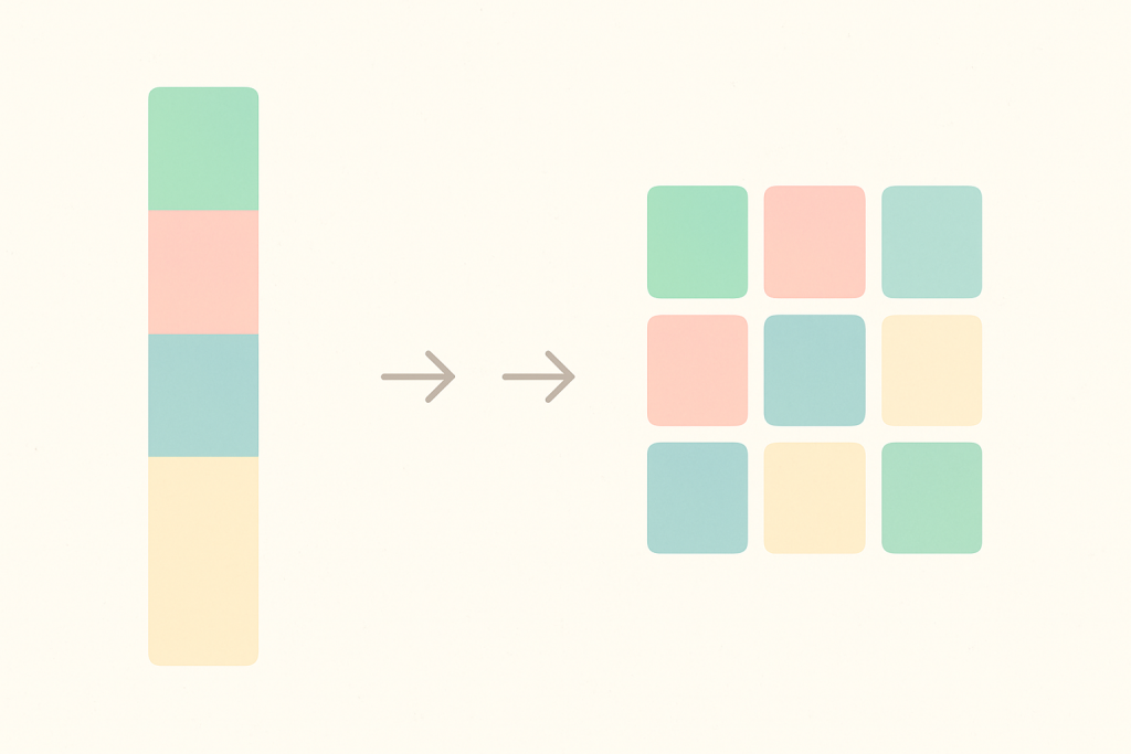
You pull a receipts export and every value lands in a single column — sixty, eighty, sometimes three hundred rows. The team wants that same list as a three-column grid for a printout, or grouped into weekly batches for review. The old fix was copy, paste-special-transpose, and hope you counted the rows right. Excel now ships two functions built for exactly this: WRAPCOLS and WRAPROWS. They take a one-dimensional list and reshape it into a two-dimensional grid, live, with one formula. Once you learn where the split falls and how the padding works, the print-ready layout is a formula rewrite away.
The sixty-second version of the syntax
Both functions take three arguments. The first is a vector — a single row or a single column, never a rectangle. The second is the wrap count: how many values before the next row or column starts. The third is optional padding for the tail cells if the vector doesn’t divide evenly. The Microsoft Learn reference for WRAPROWS documents the same signature for both, and Ablebits’ side-by-side write-up walks through a handful of the same edge cases from a different angle.
=WRAPROWS(A2:A25, 4, "")
=WRAPCOLS(A2:A25, 4, "")
A2:A25 is the vertical list of twenty-four values. 4 is the wrap count — four per row for WRAPROWS, four per column for WRAPCOLS. The empty string in the third argument fills tail cells with a blank so downstream formulas don’t trip on #N/A. Leave that third argument out and the tail cells return #N/A instead.
WRAPROWS and WRAPCOLS ship in Excel for Microsoft 365, Excel 2024, and Excel for the web. Excel 2021 does not have them; older builds fall back to INDEX plus SEQUENCE, covered later.
When a reshape actually earns its place
The functions look like a toy until you meet the layouts they solve. Three shapes come up over and over.
| Input shape | Reader wants | Formula |
|---|---|---|
| 300 names in one column | Six columns for printing | =WRAPCOLS(A2:A301, 50, "") |
| 28 daily totals in one column | Four weekly rows of seven days | =WRAPROWS(B2:B29, 7, 0) |
| 120 survey IDs in one column | Ten cohorts of twelve | =WRAPCOLS(C2:C121, 12, "") |
Each of these used to mean an ordered list, a formula for each block, and a manual splice. With one wrap call the block sizes become one argument you can change. If the source list grows from three hundred to three hundred and twenty names, the print grid updates on the next recalculation. There’s no cell-by-cell edit to catch up with the new tail.
These functions are cousins of the range-shaping crowd covered in the guide to reshaping data with CHOOSECOLS and CHOOSEROWS. The difference: CHOOSECOLS keeps the shape and picks columns from it; WRAPROWS and WRAPCOLS build the shape from a straight line.
WRAPROWS vs WRAPCOLS on the same twelve values
The two functions solve mirror problems, and the fastest way to keep them straight is to run both against the same input. Take the list 1, 2, 3, 4, 5, 6, 7, 8, 9, 10, 11, 12 in A1:A12 and wrap it four at a time.
=WRAPROWS(A1:A12, 4)

 1  2  3  4
 5  6  7  8
9 10 11 12=WRAPCOLS(A1:A12, 4)
1 5 9
2 6 10
3 7 11
4 8 12Read the outputs by row: WRAPROWS preserves the original reading order (1 through 12 left to right, top to bottom), so it’s the right call when the reader scans horizontally — a weekly calendar, a printable roster, any grid where “next” means “one cell right.”
WRAPCOLS preserves the original reading order down each column, so it’s the right call when the reader scans vertically — a phone-book layout, an alphabetical block, a two-column receipt list. Pick the function that matches the eye path, not the one whose name sounds nicer.
Padding: blank string versus #N/A
Whenever the wrap count doesn’t divide the vector evenly, the last row or column has empty tail cells. The third argument decides what fills them, and the choice matters more than it looks.
| Padding value | Downstream effect | Best for |
|---|---|---|
"" (blank string) |
Charts skip the cell. SUMIFS ignores it. Looks like an empty cell. |
Print grids, dashboards, any output shown to a person. |
0 |
Charts plot as zero. SUM unaffected. COUNTIF counts it. |
Numeric grids where a missing value truly means zero. |
omitted (default #N/A) |
Any formula reading the cell inherits the error. Loud failure. | Debugging — you want the tail cells to shout, not blend in. |
The mistake is defaulting to #N/A because “that’s what Excel does.” A single tail cell that returns #N/A will poison a chart’s axis scale, a MAX, or a downstream VLOOKUP. Pass an empty string for anything human-facing, a zero for anything summed, and only leave the padding blank when you actually want the failure to surface.
The spill trap that hits 2D output harder
Every dynamic-array function has to spill into empty cells. WRAPROWS and WRAPCOLS spill into a rectangle, not a strip, so they trip the #SPILL! error more often than SORT or FILTER ever will. A three-hundred-value wrap at ten per row needs thirty rows of clear space to land.
#SPILL! and the formula doesn’t tell you which cell got in the way — you have to hover the smart tag on the source cell to see the obstruction map.
=WRAPROWS(A2:A301, 10, "")
This formula needs cells C2:L31 completely clear. If H14 holds a stray value from an earlier experiment, the whole rectangle refuses to render. The fix is mechanical: pick a target column with genuine open space to the right and below, or clear the obstruction. For the deeper mechanics of what triggers #SPILL! and how to read the diagnostic hover, the walkthrough on fixing the Excel spill error covers each case in order.
Reversing the reshape with TOCOL and TOROW
Reshaping goes both directions. TOCOL flattens a rectangle back into a single column; TOROW flattens it into a single row. Chain either one with WRAPROWS or WRAPCOLS and you can go from list to grid and back without touching the source data.
| A | B | C | D | |
|---|---|---|---|---|
| 1 | names | grid | back to list | |
| 2 | Alex | =WRAPROWS(A2:A9,3) | =TOCOL(C2#) | |
| 3 | Blake |
The C2# operator refers to the entire spill range that starts at C2. That’s the piece that keeps this round trip live: change the wrap count in C2, the grid reshapes, and the flattened column in column D reflows to match. Pair the same idea with VSTACK and HSTACK when the source is split across several columns, and you can stitch, wrap, and flatten in one visible formula chain.
When wrapping becomes part of a real pipeline
The single-formula demos hide the real payoff. Once the wrap is live, other dynamic-array functions plug straight into it: SORT before wrapping, BYROW after wrapping, a running total across the resulting rows.
=BYROW(WRAPROWS(SORT(A2:A301), 10, ""), LAMBDA(r, SUM(r)))
This one line sorts a three-hundred-value list, wraps it into thirty rows of ten, and returns the row-wise sums as a spilled column of thirty numbers. No helper columns, no manual grouping, no macro. Change the wrap count from 10 to 15 and both the grid shape and the sum count adjust in the same tick.
Before you commit a wrap into a shared workbook, walk the checklist below. Most of the pain reports on these functions trace back to one of these five items.
- ✓ Source range is one-dimensional (single row or single column, no rectangle)
- ✓ Target has enough clear cells for the spilled rectangle
- ✓ Padding value matches what downstream formulas expect
- ✓ Wrap count is a positive integer, not a text-typed number
- ✓ Recipients are on Excel 365 or 2024 — older builds see
#NAME?
Which one belongs in your next workbook
Reach for WRAPROWS when the reader scans horizontally — a weekly calendar, a printable roster, a small results table. Reach for WRAPCOLS when the reader scans vertically — a phone-book layout, an alphabetical block, a two-column ledger. Set the wrap count once, decide what belongs in the tail cells, and the rest of the pipeline stays live.
PerRow) and reference it in the formula: =WRAPROWS(source, PerRow, ""). Reshaping the whole grid then costs one keystroke instead of a formula edit.
The next spreadsheet that arrives as a four-hundred-row column doesn’t need a manual reshape and a copy-paste-transpose ritual. It needs the right pair of arguments in a single cell.